Snapshot

Suppose an advanced alien race discovered our little planet. From their great telescopes they could tell our atmosphere is rich in oxygen and water vapor, which would indicate this was a planet inhabited by living organisms. They therefore decide to send a probe to study our curious blue world. With their advanced technology, this alien species can send a probe across the vast distance of space using a device they call the Maguffin drive. The Maguffin drive can transport the probe to Earth almost instantly, but because of the tremendous energy it requires the probe can only stay on Earth for one second.

This might seem rather pointless, but these aliens also have great scanning devices that can take images of the Earth very quickly. So they send the probe, which collects large amounts of data during its one-second visit. Many of those pictures are images of us, going about our daily lives. In essence they have taken a snapshot of our planet.

Given such a snapshot, what could these aliens possibly learn about us? It turns out quite a bit. They would know, for example, that we are social creatures, and that we tend to live in large communities. They would see that we wear clothes. They would see how we walk and run. They would also learn how we are born, live and die, and about how long we live.

Obviously a second is far too short to observe a single person be born, grow to maturity and die of old age, but there are lots of us on the planet. In that one second they would see moments of birth, children suckling at their mother’s breast, children playing, teenagers arguing with their parents, adults working and people dying. All of these moments would allow them to piece together an understanding of our lives and cultures. There’s a lot that can be gained by a snapshot.

In astronomy we do much the same things with stars. Modern astronomy has been around for only a moment on cosmological scales. We can’t possibly observe the birth, life and death of a single star. We can, however observe lots of stars at different stages. We see stars being born, stars dying, forming planets, with solar systems, etc. From all of these observations we can piece together the life cycle of a typical star.

The first step in this process is found in a graph known as the Hertzsprung-Russell (or HR) diagram. First created around 1910, this graph plotted the color of a star versus its brightness. The color was determined by measuring the apparent brightness when observed through a blue filter, and then again through a green (visible) filter. The difference between these two brightnesses is known as the B-V color index. We now know that a star’s color is determined by its surface temperature, so the color measurement was a measure of a star’s temperature.

The brightness measure was determined by measuring the apparent brightness (apparent magnitude) and the star’s distance from us. The distance is important because a bright star very far away will appear dimmer than a dim star fairly close. From a star’s distance and apparent magnitude one can determine its absolute magnitude. This is the apparent magnitude a star would have if it were 10 parsecs away. Apparent magnitude is a measure of a star’s actual brightness (or luminosity).

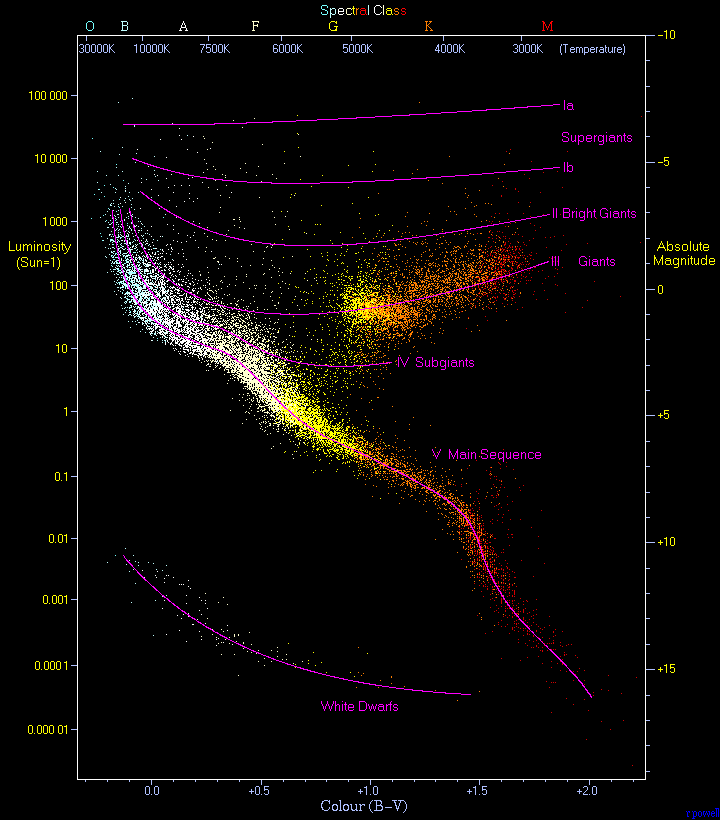Richard Powell

You can see a modern HR diagram here. One of the things you will notice is that the stars aren’t randomly distributed, but rather are clumped within certain groups. Most of the stars lay along the central diagonal line. The reddest (or coolest) stars along the line are also the dimmest, and the bluest (or hottest) stars are the brightest. This is what you would expect with a star, that cool stars are dim and hot stars are bright. Because the majority of stars lie within this region they are called main sequence stars.

But you’ll also notice a large clump of stars above the main sequence ones. These are much brighter than other stars of the same color, and they get brighter the cooler they are. At the far right of the region you have very cool stars that are also very bright. The only way for a star to be both cool and bright is for it to be very large. In other words even though it is cool compared to other stars it has much more surface area giving off light. They are therefore known as giant (or supergiant) stars.

Below the main sequence you see a scattering of dim but hot stars. To be hot but dim these stars must be quite small. Very hot, but little surface area. For this reason they are known as white dwarfs.

From such an HR diagram we can put together the life cycle of a typical star. It forms within a stellar nursery to become a main sequence star. There it spends most of its life, until it runs out of hydrogen to fuse in its core. As it begins to fuse helium it swells into a giant star, where it lives for a short time before collapsing down to a white dwarf.

We now have a very good understanding of stellar life cycles and the nuclear reactions that occur within a star. In 1910 when this diagram was first introduced we didn’t even have a complete understanding of atoms, much less nuclear physics. And yet from the beginning the diagram indicated that stars were dynamic, and that they could change over time.

All from a snapshot of the stars in our cosmic neighborhood.