The Error of My Ways

Brian Koberlein

One of the challenges of computational astrophysics is knowing how far off your answer is from the right one. Whenever you approach a problem computationally, small errors can creep in. This is similar to using 3.14 for π, or 0.33 for one third. Since computational values are finite decimals, they are usually a bit off from the exact value. You might think the answer is just to carry values out to more decimal places. While that can help, the more precise your values the more computing power it takes to calculate your problem. Often you need to strike a balance between precision and computing time/cost.

A bigger challenge is making sure your calculation errors don’t build up over time. Most computational approaches are iterative. So if you want to, say, calculate the motion of a satellite, you might calculate where it will be after 20 seconds, then use that answer to calculate the position 20 seconds after that, and so on. If your answer is a meter too far with the first step, it will be 2 meters off the second step, and so on. Your error can build with each iteration, causing what is known as error drift.

So how do you prevent error drift? One way is to look at conserved quantities (what we call invariants). To use our satellite example, we know that its energy and angular momentum are constants over time. So as you calculate the motion of the satellite with each iteration, you also calculate the energy and angular momentum. If you have error drift, then the invariants will change over time, and you know there’s a problem.

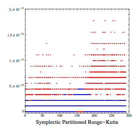
Invariants also give you a way to test the accuracy of your calculations. The less your invariants change, the better your accuracy. In the figures here, I’ve plotted the error in energy (blue) and angular momentum (red) for a simple satellite problem. In the first example, energy is held constant while the angular momentum is allowed to vary. This gives an error of only a few parts in 100 billion, which is not too shabby. In the second example, both invariants are allowed to change, but they are compared to invariants in other coordinate systems and minimized. This gives errors of a few parts in 1000 trillion, which is even better.

There are lots of different computational approaches, and each have their advantages and disadvantages. The trick is understanding those strengths and weaknesses. It’s about using the right tool for the right job.